Làm quen với Pytorch (Phần 1): Cơ bản về pytorch và bài toán Linear Regression

PyTorch là một framework được xây dựng dựa trên python cung cấp nền tảng tính toán khoa học phục vụ lĩnh vực Deep learning. Pytorch tập trung vào 2 khả năng chính:

• Một sự thay thế cho bộ thư viện numpy để tận dụng sức mạnh tính toán của GPU.
• Một platform Deep learning phục vụ trong nghiên cứu, mang lại sự linh hoạt và tốc độ.

Ưu điểm:

• Mang lại khả năng debug dễ dàng hơn theo hướng interactively, rất nhiều nhà nghiên cứu và engineer đã dùng cả pytorch và tensorflow đều đánh giá cáo pytorch hơn trong vấn đề debug và visualize.
• Hỗ trợ tốt dynamic graphs.
• Được phát triển bởi đội ngũ Facebook.
• Kết hợp cả các API cấp cao và cấp thấp.

Nhược điểm:

• Vẫn chưa được hoàn thiện trong việc deploy, áp dụng cho các hệ thống lớn,... được như framework ra đời trước nó như tensorflow.
• Ngoài document chính từ pytorch thì vẫn còn khá hạn chế các nguồn tài liệu bên ngoài như các tutorials hay các câu hỏi trên stackoverflow.

Ma trận

• Trong pytorch, ma trận(mảng) được gọi là các tensors.
• Ma trận 2 chiều 3 * 3 được gọi là 3 * 3 tensor.
• Cùng nhìn lại ví dụ về mảng(array) với numpy mà chúng ta đều đã biết:

1. Ta tạo numpy array với hàm np.array()
2. Type(): type của array. Trong ví dụ này đó là kiểu numpy.
3. np.shape(): kính cỡ của array. Hàng x Cột

# import numpy library
import numpy as np

# numpy array
array = [[1,2,3],[4,5,6]]
first_array = np.array(array) # 2x3 array
print("Array Type: {}".format(type(first_array))) # type
print("Array Shape: {}".format(np.shape(first_array))) # shape
print(first_array)

output:

Array Type: <class 'numpy.ndarray'>
Array Shape: (2, 3)
[[1 2 3]
 [4 5 6]]

Chúng ta đã hiểu qua về numpy array giờ hãy cùng xem cách implement tensor array(pytorch array).

• Thêm thư viện pytorch bằng dòng code: import torch
• Chúng ta tạo tensor với hàm torch.Tensor().
• type: Kiểu array. Trong ví dụ này là tensor.
• shape: kích cỡ của array. Hàng x Cột

# import pytorch library
import torch

# pytorch array
tensor = torch.Tensor(array)
print("Array Type: {}".format(tensor.type)) # type
print("Array Shape: {}".format(tensor.shape)) # shape
print(tensor)

output:

Array Type: <bound method _type of 
 1  2  3
 4  5  6
[torch.FloatTensor of size 2x3]
>
Array Shape: torch.Size([2, 3])

 1  2  3
 4  5  6
[torch.FloatTensor of size 2x3]

Phân phối là một trong những kĩ thuật được sử dụng nhiều nhất trong coding. Hãy cùng xem cách làm nó trong pytorch.

Hãy cùng so sánh numpy và tensor:

• np.ones() = torch.ones()
• np.random.rand() = torch.rand()

# numpy ones
print("Numpy {}
".format(np.ones((2,3))))

# pytorch ones
print(torch.ones((2,3)))

output:

Numpy [[1. 1. 1.]
 [1. 1. 1.]]


 1  1  1
 1  1  1
[torch.FloatTensor of size 2x3]

Với tensor:

# numpy random
print("Numpy {}
".format(np.random.rand(2,3)))

# pytorch random
print(torch.rand(2,3))

output:

Numpy [[0.18841978 0.61702582 0.95432382]
 [0.16407638 0.18776019 0.52468443]]


 0.3779  0.3206  0.8350
 0.4805  0.5554  0.2068
[torch.FloatTensor of size 2x3]

Kể cả khi tôi sử dụng pytorch cho neural networks, tôi vẫn cảm thấy tốt hơn khi sử dụng numpy. Vì thế mà tôi thường xuyên convert kết quả của neural network từ tensor sang numpy array để visualize hoặc đánh giá.

Hãy cùng xem cách chuyển qua lại giữa tensor và numpy array:

• torch.from_numpy(): từ numpy sang tensor
• numpy(): từ tensor sang numpy

# random numpy array
array = np.random.rand(2,2)
print("{} {}
".format(type(array),array))

# from numpy to tensor
from_numpy_to_tensor = torch.from_numpy(array)
print("{}
".format(from_numpy_to_tensor))

# from tensor to numpy
tensor = from_numpy_to_tensor
from_tensor_to_numpy = tensor.numpy()
print("{} {}
".format(type(from_tensor_to_numpy),from_tensor_to_numpy))

output:

<class 'numpy.ndarray'> [[0.93007643 0.87933967]
 [0.99716134 0.69613825]]


 0.9301  0.8793
 0.9972  0.6961
[torch.DoubleTensor of size 2x2]


<class 'numpy.ndarray'> [[0.93007643 0.87933967]
 [0.99716134 0.69613825]]

Toán học cơ bản với pytorch

• Resize: view()
• a và b là tensor.
• Phép cộng: torch.add(a,b) = a + b
• Phép trừ: a.sub(b) = a - b
• Phép nhân tương ứng từng phần tử: torch.mul(a,b) = a * b
• Phép chia tương ứng từng phần tử: torch.div(a,b) = a / b
• Mean: a.mean()
• Độ lệch tiêu chuẩn (std): a.std()

# create tensor 
tensor = torch.ones(3,3)
print("
",tensor)

# Resize
print("{}{}
".format(tensor.view(9).shape,tensor.view(9)))

# Addition
print("Addition: {}
".format(torch.add(tensor,tensor)))

# Subtraction
print("Subtraction: {}
".format(tensor.sub(tensor)))

# Element wise multiplication
print("Element wise multiplication: {}
".format(torch.mul(tensor,tensor)))

# Element wise division
print("Element wise division: {}
".format(torch.div(tensor,tensor)))

# Mean
tensor = torch.Tensor([1,2,3,4,5])
print("Mean: {}".format(tensor.mean()))

# Standart deviation (std)
print("std: {}".format(tensor.std()))

output:

1  1  1
 1  1  1
 1  1  1
[torch.FloatTensor of size 3x3]

torch.Size([9])
 1
 1
 1
 1
 1
 1
 1
 1
 1
[torch.FloatTensor of size 9]


Addition: 
 2  2  2
 2  2  2
 2  2  2
[torch.FloatTensor of size 3x3]


Subtraction: 
 0  0  0
 0  0  0
 0  0  0
[torch.FloatTensor of size 3x3]


Element wise multiplication: 
 1  1  1
 1  1  1
 1  1  1
[torch.FloatTensor of size 3x3]


Element wise division: 
 1  1  1
 1  1  1
 1  1  1
[torch.FloatTensor of size 3x3]


Mean: 3.0
std: 1.5811388300841898

Variables

Nếu các bạn chưa có kiến thức về backpropagation hay gradient thì các bạn nên đọc bài viết về neural network của mình tại đây để có thể hiểu được các phần tiếp theo.

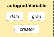
Variable là class bao bọc (wrapper) Tensor cho phép thực hiện tính toán đạo hàm. Variable lưu trữ data (tensor) và grad (gradient).

# import variable from pytorch library
from torch.autograd import Variable

# define variable
var = Variable(torch.ones(3), requires_grad = True)
var

output:

Variable containing:
 1
 1
 1
[torch.FloatTensor of size 3]

• Giả sử ta có phương trình y = x^2
• Định nghĩa variable x = [2,4]
• Sau khi tính toán ta được y = [4,16] (y = x^2)
• Phương trình o: o = (1/2)sum(y) = (1/2)sum(x^2)
• Đạo hàm của o = x
• Kết qủa bằng x nên gradients là [2,4]

# lets make basic backward propagation
# we have an equation that is y = x^2
array = [2,4]
tensor = torch.Tensor(array)
x = Variable(tensor, requires_grad = True)
y = x**2
print(" y =  ",y)

# recap o equation o = 1/2*sum(y)
o = (1/2)*sum(y)
print(" o =  ",o)

# backward
o.backward() # calculates gradients

# As I defined, variables accumulates gradients. In this part there is only one variable x.
# Therefore variable x should be have gradients
# Lets look at gradients with x.grad
print("gradients: ",x.grad)

output:

y =   Variable containing:
  4
 16
[torch.FloatTensor of size 2]

 o =   Variable containing:
 10
[torch.FloatTensor of size 1]

gradients:  Variable containing:
 2
 4
[torch.FloatTensor of size 2]

Autograd

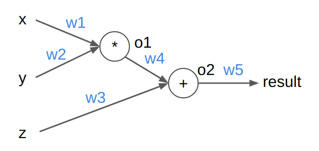
Minh họa cách tính Gradient tự động trong Pytorch bằng ví dụ sau: Cho đồ thị tính toán như hình. Đầu vào [x,y,z] = [5,3,7]. Tất cả các trọng số w đều được khởi tạo là 0.5. Tính kết quả (biến result) khi ta cho [x,y,z] qua mạng (forward) và gradient của mỗi trọng số w (backward).

import torch
from torch.autograd import Variable

xy = Variable(torch.FloatTensor([5, 3]), requires_grad=True) # size: 2
z = Variable(torch.FloatTensor([7]), requires_grad=True)    # size: 1
w12 = Variable(torch.FloatTensor([0.5, 0.5]), requires_grad=True)   # size: 2
w3 = Variable(torch.FloatTensor([0.5]), requires_grad=True) # size: 1
w4 = Variable(torch.FloatTensor([0.5]), requires_grad=True) # size: 1
w5 = Variable(torch.FloatTensor([0.5]), requires_grad=True) # size: 1

k = xy*w12
o1 = k[0]*k[1]
o2 = o1*w4 + z*w3
result = o2*w5
print('result', result)         # 2.6875

result.backward()
print('w12.grad', w12.grad)     # 1.8750, 1.8750
print('w3.grad', w3.grad)       # 3.5000
print('w4.grad', w4.grad)       # 1.8750
print('w5.grad', w5.grad)       # 5.3750

Giải thích :

Forward:

o1 = x * w1 * y * w2 = 5 * 0.5 * 3 * 0.5 = 3.75

o2 = o1 * w4 + z * w3 = 3.75 * 0.5 + 7 * 0.5 = 5.375

result = o2 * w5 = 5.375 * 0.5 = 2.6875

Backward:

Cần chú ý công thức đạo hàm của hàm hợp:

f'(u(x)) = f'(u) * u'(x)

result = o2 * w5

Đạo hàm của result theo w5 = (o2 * w5)' = o2 = 5.375

Đạo hàm của result theo o2 = f'(o2) = w5 = 0.5

o2 = o1 * w4 + z * w3

Đạo hàm của result theo w3 = f'(o2) * o2'(w3) = 0.5 * z = 3.5

Đạo hàm của result theo w4 = f'(o2) * o2'(w4) = 0.5 * o1 = 1.875

Đạo hàm của result theo o1 = g'(o1) = f'(o2) * o2'(o1) = 0.5 * w4 = 0.25

o1 = x * w1 * y * w2

Đạo hàm của result theo w1 = g'(o1) * o1'(w1) = 0.25 * x * y * w2 = 1.875

Đạo hàm của result theo w2 = g'(o1) * o1'(w2) = 0.25 * x * w1 * y = 1.875

Linear Regression

Nếu các bạn chưa có kiến thức về Linear Regression thì có thể tham khảo tại đây.

• Hàm y = Ax + B.
• Ví dụ: giả sử chúng ta có một công ty ô tô. Nếu giá xe xuống thấp, chúng ta sẽ bán được nhiều xe hơn. Nếu giá xe tăng cao, ta bán được ít xe hơn. Đây là thực tế mà chúng ta biết và chúng ta có dữ liệu về điều này.
• Câu hỏi đặt ra là làm sao để ước lượng được số xe ta sẽ bán được khi mà giá xe là 100.

# As a car company we collect this data from previous selling
# lets define car prices
car_prices_array = [3,4,5,6,7,8,9]
car_price_np = np.array(car_prices_array,dtype=np.float32)
car_price_np = car_price_np.reshape(-1,1)
car_price_tensor = Variable(torch.from_numpy(car_price_np))

# lets define number of car sell
number_of_car_sell_array = [ 7.5, 7, 6.5, 6.0, 5.5, 5.0, 4.5]
number_of_car_sell_np = np.array(number_of_car_sell_array,dtype=np.float32)
number_of_car_sell_np = number_of_car_sell_np.reshape(-1,1)
number_of_car_sell_tensor = Variable(torch.from_numpy(number_of_car_sell_np))

# lets visualize our data
import matplotlib.pyplot as plt
plt.scatter(car_prices_array,number_of_car_sell_array)
plt.xlabel("Car Price $")
plt.ylabel("Number of Car Sell")
plt.title("Car Price$ VS Number of Car Sell")
plt.show()

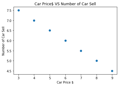
Hình trên ta đã plot dữ liệu mà ta thu thập được và câu hỏi đặt ra là tìm số lượng xe sẽ bán được khi giá ô tô là 100. Để trả lời câu hỏi này ta sẽ cần sử dụng Linear Regression. Về cơ bản chúng ta sẽ cố tạo ra một đường thẳng fit với dữ liệu đã được plot ở trên và cố gắng tinh chỉnh đường thẳng đó sao cho giảm được độ lệch vs data.

Các bước thực hiện Linear Regression

• Tạo lớp LinearRegression
• Tạo model trong class LinearRegression
• MSE: Mean squared error
• Optimization (SGD:stochastic gradient descent)
• Backpropagation
• Đưa ra dự đoán

# Linear Regression with Pytorch

# libraries
import torch      
from torch.autograd import Variable     
import torch.nn as nn 
import warnings
warnings.filterwarnings("ignore")

# create class
class LinearRegression(nn.Module):
    def __init__(self,input_size,output_size):
        # super function. It inherits from nn.Module and we can access everythink in nn.Module
        super(LinearRegression,self).__init__()
        # Linear function.
        self.linear = nn.Linear(input_dim,output_dim)

    def forward(self,x):
        return self.linear(x)
    
# define model
input_dim = 1
output_dim = 1
model = LinearRegression(input_dim,output_dim) # input and output size are 1

# MSE
mse = nn.MSELoss()

# Optimization (find parameters that minimize error)
learning_rate = 0.02   # how fast we reach best parameters
optimizer = torch.optim.SGD(model.parameters(),lr = learning_rate)

# train model
loss_list = []
iteration_number = 1001
for iteration in range(iteration_number):
        
    # optimization
    optimizer.zero_grad() 
    
    # Forward to get output
    results = model(car_price_tensor)
    
    # Calculate Loss
    loss = mse(results, number_of_car_sell_tensor)
    
    # backward propagation
    loss.backward()
    
    # Updating parameters
    optimizer.step()
    
    # store loss
    loss_list.append(loss.data)
    
    # print loss
    if(iteration % 50 == 0):
        print('epoch {}, loss {}'.format(iteration, loss.data))

plt.plot(range(iteration_number),loss_list)
plt.xlabel("Number of Iterations")
plt.ylabel("Loss")
plt.show()

output:

epoch 0, loss 
 10.2133
[torch.FloatTensor of size 1]

epoch 50, loss 
 5.6256
[torch.FloatTensor of size 1]

epoch 100, loss 
 3.8014
[torch.FloatTensor of size 1]

epoch 150, loss 
 2.5688
[torch.FloatTensor of size 1]

epoch 200, loss 
 1.7358
[torch.FloatTensor of size 1]

epoch 250, loss 
 1.1730
[torch.FloatTensor of size 1]

epoch 300, loss 
 0.7926
[torch.FloatTensor of size 1]

epoch 350, loss 
 0.5356
[torch.FloatTensor of size 1]

epoch 400, loss 
 0.3619
[torch.FloatTensor of size 1]

epoch 450, loss 
 0.2446
[torch.FloatTensor of size 1]

epoch 500, loss 
 0.1653
[torch.FloatTensor of size 1]

epoch 550, loss 
 0.1117
[torch.FloatTensor of size 1]

epoch 600, loss 
1.00000e-02 *
  7.5467
[torch.FloatTensor of size 1]

epoch 650, loss 
1.00000e-02 *
  5.0996
[torch.FloatTensor of size 1]

epoch 700, loss 
1.00000e-02 *
  3.4460
[torch.FloatTensor of size 1]

epoch 750, loss 
1.00000e-02 *
  2.3286
[torch.FloatTensor of size 1]

epoch 800, loss 
1.00000e-02 *
  1.5735
[torch.FloatTensor of size 1]

epoch 850, loss 
1.00000e-02 *
  1.0633
[torch.FloatTensor of size 1]

epoch 900, loss 
1.00000e-03 *
  7.1854
[torch.FloatTensor of size 1]

epoch 950, loss 
1.00000e-03 *
  4.8554
[torch.FloatTensor of size 1]

epoch 1000, loss 
1.00000e-03 *
  3.2808
[torch.FloatTensor of size 1]

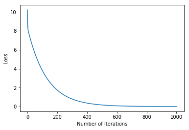
• Số vòng lặp là 1001.
• Bạn có thể thấy từ epoch 1000 loss đã gần như bằng 0
• Như vậy bây giờ ta đã có một model đã được huấn luyện
• Và giờ thì dùng model đó để dự đoán cho bài toán của chúng ta thôi

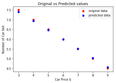
# predict our car price 
predicted = model(car_price_tensor).data.numpy()
plt.scatter(car_prices_array,number_of_car_sell_array,label = "original data",color ="red")
plt.scatter(car_prices_array,predicted,label = "predicted data",color ="blue")

# predict if car price is 10$, what will be the number of car sell
#predicted_10 = model(torch.from_numpy(np.array([10]))).data.numpy()
#plt.scatter(10,predicted_10.data,label = "car price 10$",color ="green")
plt.legend()
plt.xlabel("Car Price $")
plt.ylabel("Number of Car Sell")
plt.title("Original vs Predicted values")
plt.show()

Mình hy vọng với phần 1 này các bạn đã làm quen được với pytorch và có thể tự mình code thành thục được một số chức năng cơ bản. Ở phần 2 chúng ta sẽ đi vào tìm hiểu cách implement pytorch cho một số mô hình deep learning.

• https://www.kaggle.com/kanncaa1/pytorch-tutorial-for-deep-learning-lovers
• https://minhng.info/ai/pytorch-co-ban.html