Time Complexity For Ruby Developers
When we talk about time complexity in computer science, the first thing that we programmers mention is Big O notation which specifically describes the worst-case or best-case scenario. We use it to describe the execution time required or the space used (e.g. in memory or on disk) by an algorithm. ...
When we talk about time complexity in computer science, the first thing that we programmers mention is Big O notation which specifically describes the worst-case or best-case scenario. We use it to describe the execution time required or the space used (e.g. in memory or on disk) by an algorithm. It’s interesting because it helps us see why a particular algorithm or program may be slow & what can we do to make it faster. We need to know first what is slow & what is fast. For instance, Is sorting 1 million numbers in 150ms (milliseconds) slow or fast?
Big O Notation and Complexity
Big O Notation tells us how complex is an algorithm depending on what we feed it. The important thing to understand with the Big O notation is that it only cares about the worst case scenario.
Here are a few examples of different complexities.
With Big O notation we can classify algorithms according to their performance.
O(1)O(1) represents a “constant time” algorithm. That means that the algorithm will always take the same time to finish its work, regardless of how much work it has to do.
def first_element_is_red?(array)
  array[0] =='red' ? true : false
end
O(n)
O(n) means that the execution time of an algorithm will grow linearly depending on the input size.
def contains?(array, value)
  array.each do |item|
    return true if item == value
  end
  false
end
Here the Big O only cares about the worst case, right? In this example, we could find the value in the first iteration… or not find it at all, which would be the worst case. That’s why this algorithm has a complexity of O(n). Here’s a table:
| Notation | Name | Description |
|---|---|---|
| O(1) | Constant | Always takes same time |
| O(log n) | Logarithmic | Amount of work is divided by 2 after every loop iteration (binary search). |
| O(n) | Linear | Time to complete the work grows in a 1 to 1 relation to input size |
| O(n log n) | Linearithmic | This is a nested loop, where the inner loop runs in log n time. Examples include quicksort, mergesort & heapsort |
| O(n^2) | Quadratic | Time to complete the work grows in a input size ^ 2 relation. You can recognize this whenever you have a loop that goes over all the elements & every iteration of the loop also goes over every element. You have a nested loop. |
| O(n^3) | Cubic | Same as n^2, but time grows in a n^3 relation to input size. Look for a triple nested loop to recognize this one. |
| O(2^n) | Exponential | Time to complete the work grows in a 2 ^ input size relation. This is a lot slower than n^2, so don’t confuse them! One example is the recursive fibonacci algorithm |
Algorithm Analysis
We can start developing our intuition for this if we think about the input as an array of “n” elements.
Imagine that we want to find all the elements that are odd numbers, the only way to do this is to read every element once to see if it matches the condition.
[1,2,3,4,5,6,7,8,9,10].select(&:odd?)
We can’t skip numbers because we may miss some of the numbers we are looking for, so that makes this a linear time algorithm O(n)
Good Algorithms are Fast Algorithms
We are going to explore 3 code examples for a Scrabble solution checker to have an idea about what algorithm is likely to perform better.
Scrabble is a game that given a list of characters (like lordw) asks you to form words (like world) using these characters.
Here’s the first solution:
def scramble(chars, word)
  word.each_char.all? { |c| chars.count(c) >= word.count(c) }
end
How can we know what is the time complexity of this code? The key is in the count method, so make sure you understand what that method does.
The answer is: O(n^2).
And the reason for that is that with each_char we are going over all the characters in the string word. That alone would be a linear time algorithm O(n), but inside the block we have the count method.
This method is actually another loop which goes over all the characters in the string again to count them.
It's Ok but how can we do better? Is there a way to avoid some looping?
Instead of counting the characters we could remove them, that way we have less characters to go through.
Here’s the second solution:
def scramble(chars, word)
  characters = chars.dup
  word.each_char.all? { |c| characters.sub!(c, "") }
end
This one is a different. This will be a lot faster than the count version in the best case, where the characters we are looking for are near the start of the string.
But when the characters are all at the end, in reverse order of how they are in found in word, the performance will be similar to that of the count version, so we can say that this is still an O(n^2) algorithm
We don’t have to worry about the case where none of the characters in word are available, because the all? method will stop as soon as sub! returns false. But you would only know this if you have studied Ruby extensively.
Let’s try with one more solution.
What if we remove any kind of looping inside the block? We can do that with a hash.
def scramble(chars, word)
  available = Hash.new(1)
  chars.each_char { |c| available[c] += 1 }
  word.each_char.all? { |c| available[c] -= 1; available[c] > 0 }
end
Reading & writing hash values is a O(1) operation, which means it’s pretty fast, especially compared to looping.
We still have two loops, one to build the hash table, and one to check it. Because these loops aren’t nested this is an O(n) algorithm.
If we benchmark these 3 solutions we can see that our analysis matches with the results:
hash    1.216667   0.000000   1.216667 (  1.216007)
sub     6.240000   1.023333   7.263333 (  7.268173)
count 222.866644   0.073333 222.939977 (223.440862)
Here’s a line chart:
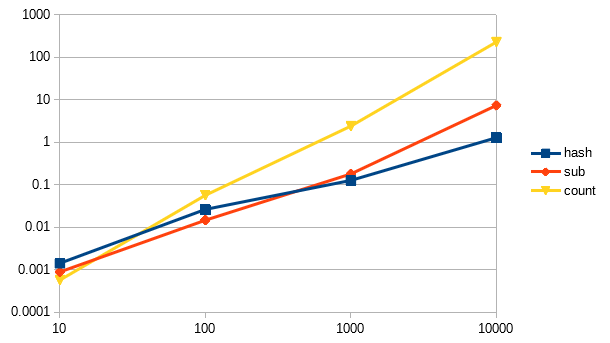
We can notice a few things, The Y axis (vertical) represents how many seconds it took to complete the work, while the X axis (horizontal) represents the input size. This is a logarithmic chart, which compresses the values in a certain range, but in reality the count line is a lot steeper. This logarithmic chart tell us with a very smaller input size count is actually faster!
Summary
We now have a basic idea about algorithmic time complexity, big O notation & time complexity analysis. We saw some examples where we compare different solutions to the same problem & analyzed their performance.