Làm quen với Pytorch (Phần 2): Bài toán phân loại và Deeplearning
Logistic Regression Linear regression mà ta đã biết ở phần 1 không sử dụng được cho bài toàn phân loại, vậy nên chúng ta cần phải sử dụng Logistic regression. Về cơ bản thì logistic regression = linear regression + logistic function. Nếu bạn chưa có kiến thức cơ bản về logistic regression thì có ...
Logistic Regression
Linear regression mà ta đã biết ở phần 1 không sử dụng được cho bài toàn phân loại, vậy nên chúng ta cần phải sử dụng Logistic regression. Về cơ bản thì logistic regression = linear regression + logistic function. Nếu bạn chưa có kiến thức cơ bản về logistic regression thì có thể đọc tại đây.
Các bước của Logistic regression:
- Import thư viện.
- Chuẩn bị dataset:
- Sử dụng bộ MNIST dataset
- Chứa các ảnh với kích thước 28 * 28 và 10 labels từ 0 đến 9.
- Data chưa được normalized nên ta cần chia mọi pixels của ảnh cho 255 để đưa dữ liệu về khoảng [0,1], đây là một bước xử lý cơ bản cho ảnh.
- Để chia dữ liệu train và test ta sử dụng hàm train_test_split trong thư viện sklearn.
- Ta sẽ chia kích thước của train data là 80% và của test data là 20%.
- Tạo các features và tensors.
- batch_size: Ví dụ ta có một dataset chứa 1000 sample. Ta có thể train 1000 sample cùng một lúc hoặc ta có thể chia ra 10 nhóm mỗi nhóm chứa 100 sample. Batch size chính là kích thước của mỗi nhóm, trong trường hợp này là 100.
- epoch: 1 epoch có nghĩa là training tất cả sample trong 1 lần.
- Ví dụ: ta có 33600 sample để train và ta chọn batch_size = 100. Đồng thời ta cũng chọn epoch là 29. Data sẽ được train 29 lần. Câu hỏi đặt ra là cần bao nhiêu vòng lặp là đủ? Tính thử xem: training data 1 lần = training 33600 sample (vì data chứa 33600 sample). Nhưng ta đã chia data ra thành 336 nhóm(batch_size = 100). Vậy nên 1 epoch sẽ gồm 336 vòng lặp. Ta có 29 epoch nên tổng số vòng lặp sẽ là 336 * 29 = 9744.
- TensorDataset(): đây là Dataset wrapping tensors. Các sample được lấy dựa vào indexing tensors dọc theo chiều đầu tiên của tensor.
- DataLoader(): Nó giúp kết hợp dataset and sampler. Và nó cũng cung cấp đa xử lý vòng lặp qua bộ dataset.
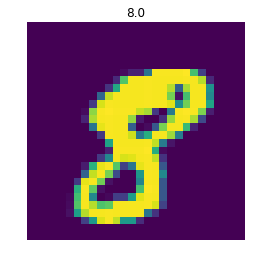
- Visualize 1 ảnh trong dataset.
- Tạo Logistic Regression Model
- Giống với linear regression.
- Tuy nhiên cần phải thêm ligistic function.
- Trong pytorch, logistic function nằm trong loss function.
- Khởi tạo Model Class
- input_dim = 28 * 28 # size của images
- output_dim = 10 # labels 0,1,2,3,4,5,6,7,8,9
- tạo model
- Khởi tạo Loss Class
- Ta sử dụng Cross entropy loss.
- Nó cũng chứa softmax(logistic function).
- Optimizer Class
- SGD Optimizer
- Traning Model
- Prediction
# Import Libraries
import torch
import torch.nn as nn
import torchvision.transforms as transforms
from torch.autograd import Variable
import pandas as pd
from sklearn.model_selection import train_test_split
# Prepare Dataset
# load data
train = pd.read_csv(r"../input/train.csv",dtype = np.float32)

# split data into features(pixels) and labels(numbers from 0 to 9)
targets_numpy = train.label.values
features_numpy = train.loc[:,train.columns != "label"].values/255 # normalization

# train test split. Size of train data is 80% and size of test data is 20%.
features_train, features_test, targets_train, targets_test = train_test_split(features_numpy,
                                                                             targets_numpy,
                                                                             test_size = 0.2,
                                                                             random_state = 42)

# create feature and targets tensor for train set. As you remember we need variable to accumulate gradients. Therefore first we create tensor, then we will create variable
featuresTrain = torch.from_numpy(features_train)
targetsTrain = torch.from_numpy(targets_train).type(torch.LongTensor) # data type is long

# create feature and targets tensor for test set.
featuresTest = torch.from_numpy(features_test)
targetsTest = torch.from_numpy(targets_test).type(torch.LongTensor) # data type is long

# batch_size, epoch and iteration
batch_size = 100
n_iters = 10000
num_epochs = n_iters / (len(features_train) / batch_size)
num_epochs = int(num_epochs)

# Pytorch train and test sets
train = torch.utils.data.TensorDataset(featuresTrain,targetsTrain)
test = torch.utils.data.TensorDataset(featuresTest,targetsTest)

# data loader
train_loader = torch.utils.data.DataLoader(train, batch_size = batch_size, shuffle = False)
test_loader = torch.utils.data.DataLoader(test, batch_size = batch_size, shuffle = False)

# visualize one of the images in data set
plt.imshow(features_numpy[10].reshape(28,28))
plt.axis("off")
plt.title(str(targets_numpy[10]))
plt.savefig('graph.png')
plt.show()
# Create Logistic Regression Model
class LogisticRegressionModel(nn.Module):
    def __init__(self, input_dim, output_dim):
        super(LogisticRegressionModel, self).__init__()
        # Linear part
        self.linear = nn.Linear(input_dim, output_dim)
        # There should be logistic function right?
        # However logistic function in pytorch is in loss function
        # So actually we do not forget to put it, it is only at next parts

    def forward(self, x):
        out = self.linear(x)
        return out

# Instantiate Model Class
input_dim = 28*28 # size of image px*px
output_dim = 10  # labels 0,1,2,3,4,5,6,7,8,9

# create logistic regression model
model = LogisticRegressionModel(input_dim, output_dim)

# Cross Entropy Loss
error = nn.CrossEntropyLoss()

# SGD Optimizer
learning_rate = 0.001
optimizer = torch.optim.SGD(model.parameters(), lr=learning_rate)
# Traning the Model
count = 0
loss_list = []
iteration_list = []
for epoch in range(num_epochs):
    for i, (images, labels) in enumerate(train_loader):

        # Define variables
        train = Variable(images.view(-1, 28*28))
        labels = Variable(labels)

        # Clear gradients
        optimizer.zero_grad()

        # Forward propagation
        outputs = model(train)

        # Calculate softmax and cross entropy loss
        loss = error(outputs, labels)

        # Calculate gradients
        loss.backward()

        # Update parameters
        optimizer.step()

        count += 1

        # Prediction
        if count % 50 == 0:
            # Calculate Accuracy
            correct = 0
            total = 0
            # Predict test dataset
            for images, labels in test_loader:
                test = Variable(images.view(-1, 28*28))

                # Forward propagation
                outputs = model(test)

                # Get predictions from the maximum value
                predicted = torch.max(outputs.data, 1)[1]

                # Total number of labels
                total += len(labels)

                # Total correct predictions
                correct += (predicted == labels).sum()

            accuracy = 100 * correct / float(total)

            # store loss and iteration
            loss_list.append(loss.data)
            iteration_list.append(count)
        if count % 500 == 0:
            # Print Loss
            print('Iteration: {}  Loss: {}  Accuracy: {}%'.format(count, loss.data, accuracy))
output :
Iteration: 500  Loss:
 1.8170
[torch.FloatTensor of size 1]
  Accuracy: 65.94047619047619%
Iteration: 1000  Loss:
 1.5917
[torch.FloatTensor of size 1]
  Accuracy: 73.78571428571429%
Iteration: 1500  Loss:
 1.2932
[torch.FloatTensor of size 1]
  Accuracy: 77.75%
Iteration: 2000  Loss:
 1.2070
[torch.FloatTensor of size 1]
  Accuracy: 79.76190476190476%
Iteration: 2500  Loss:
 1.0171
[torch.FloatTensor of size 1]
  Accuracy: 81.0%
Iteration: 3000  Loss:
 0.9256
[torch.FloatTensor of size 1]
  Accuracy: 81.67857142857143%
Iteration: 3500  Loss:
 0.9007
[torch.FloatTensor of size 1]
  Accuracy: 82.39285714285714%
Iteration: 4000  Loss:
 0.7440
[torch.FloatTensor of size 1]
  Accuracy: 82.95238095238095%
Iteration: 4500  Loss:
 0.9708
[torch.FloatTensor of size 1]
  Accuracy: 83.4047619047619%
Iteration: 5000  Loss:
 0.8124
[torch.FloatTensor of size 1]
  Accuracy: 83.79761904761905%
Iteration: 5500  Loss:
 0.7532
[torch.FloatTensor of size 1]
  Accuracy: 84.07142857142857%
Iteration: 6000  Loss:
 0.8698
[torch.FloatTensor of size 1]
  Accuracy: 84.41666666666667%
Iteration: 6500  Loss:
 0.6617
[torch.FloatTensor of size 1]
  Accuracy: 84.67857142857143%
Iteration: 7000  Loss:
 0.7158
[torch.FloatTensor of size 1]
  Accuracy: 84.86904761904762%
Iteration: 7500  Loss:
 0.6394
[torch.FloatTensor of size 1]
  Accuracy: 85.04761904761905%
Iteration: 8000  Loss:
 0.7324
[torch.FloatTensor of size 1]
  Accuracy: 85.27380952380952%
Iteration: 8500  Loss:
 0.5474
[torch.FloatTensor of size 1]
  Accuracy: 85.4047619047619%
Iteration: 9000  Loss:
 0.6534
[torch.FloatTensor of size 1]
  Accuracy: 85.52380952380952%
Iteration: 9500  Loss:
 0.5278
[torch.FloatTensor of size 1]
  Accuracy: 85.64285714285714%
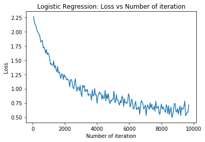
# visualization
plt.plot(iteration_list,loss_list)
plt.xlabel("Number of iteration")
plt.ylabel("Loss")
plt.title("Logistic Regression: Loss vs Number of iteration")
plt.show()
Artificial Neural Network (ANN)
Logistic regression khá tốt trong classification nhưng khi độ phức tạp tăng lên, độ chính xác của model giảm đi. Do đó, chúng ta cần tăng độ phức tạp của model. Để làm điều đó, ta cần thêm các non-linear functions vào các hidden layers. Điều ta nhận ra từ NN là khi độ phức tạp tăng lên, nếu dùng thêm các hidden layers thì model của chúng ta càng tốt lên, từ đó độ chính xác tăng lên.
Để đọc bài viết này được tốt hơn thì bạn cần phải có kiến thức cơ bản về Neural network. Nếu bạn chưa biết Neural network là gì thì bạn có thể đọc về nó tại đây hoặc bài viết trên kaggle tại đây. Tôi sẽ không đi vào việc giải thích lại về NN mà sẽ chỉ đi vào vấn đề chính là implement pytorch cho Neural network.
Neural network là một phần quan trọng nhất trong bài viết này. Nếu bạn có thể hiểu tốt phần này thì những phần tiếp theo về CNN hay RNN sẽ vô cùng dễ dàng.
Các bước implement ANN:
- Import thư viện
- Xử lý Dataset
- Hoàn toàn giống như phần trước(logistic regression).
- Chúng ta sử dụng bộ data như cũ nên ta chỉ cần train_loader và test_loader.
- Ta sử dụng batch size, epoch và số vòng lặp như cũ.
- Tạo ANN Model
- Thêm 3 hidden layers.
- Sử dụng ReLU, Tanh và ELU activation functions để giúp tăng sự đa dạng.
- Khởi tạo Model Class
- input_dim = 2828 # size của ảnh
- output_dim = 10 # labels 0,1,2,3,4,5,6,7,8,9
- Hidden layer có chiều is 150. Tôi chỉ chọn nó là 150 và thực sự là chẳng có bí quyết hay lý do nào cả. Thực sự thì số unit của hidden layer là hyperparameter và nó được chọn và điều chỉnh. Bạn có thể thử số chiều khác cho hidden layer và quan sát kết quả.
- Tạo model
- Loss Class
- Sử dụng Cross entropy loss
- Và nó cũng chứa softmax(logistic function).
- Optimizer Class
- SGD Optimizer
- Traning Model
- Prediction
# Import Libraries
import torch
import torch.nn as nn
import torchvision.transforms as transforms
from torch.autograd import Variable
# Create ANN Model
class ANNModel(nn.Module):
    def __init__(self, input_dim, hidden_dim, output_dim):
        super(ANNModel, self).__init__()
        # Linear function 1: 784 --> 100
        self.fc1 = nn.Linear(input_dim, hidden_dim)
        # Non-linearity 1
        self.relu1 = nn.ReLU()

        # Linear function 2: 100 --> 100
        self.fc2 = nn.Linear(hidden_dim, hidden_dim)
        # Non-linearity 2
        self.tanh2 = nn.Tanh()

        # Linear function 3: 100 --> 100
        self.fc3 = nn.Linear(hidden_dim, hidden_dim)
        # Non-linearity 3
        self.elu3 = nn.ELU()

        # Linear function 4 (readout): 100 --> 10
        self.fc4 = nn.Linear(hidden_dim, output_dim)

    def forward(self, x):
        # Linear function 1
        out = self.fc1(x)
        # Non-linearity 1
        out = self.relu1(out)

        # Linear function 2
        out = self.fc2(out)
        # Non-linearity 2
        out = self.tanh2(out)

        # Linear function 2
        out = self.fc3(out)
        # Non-linearity 2
        out = self.elu3(out)

        # Linear function 4 (readout)
        out = self.fc4(out)
        return out

# instantiate ANN
input_dim = 28*28
hidden_dim = 150 #hidden layer dim is one of the hyper parameter and it should be chosen and tuned. For now I only say 150 there is no reason.
output_dim = 10

# Create ANN
model = ANNModel(input_dim, hidden_dim, output_dim)

# Cross Entropy Loss
error = nn.CrossEntropyLoss()

# SGD Optimizer
learning_rate = 0.02
optimizer = torch.optim.SGD(model.parameters(), lr=learning_rate)
# ANN model training
count = 0
loss_list = []
iteration_list = []
accuracy_list = []
for epoch in range(num_epochs):
    for i, (images, labels) in enumerate(train_loader):

        train = Variable(images.view(-1, 28*28))
        labels = Variable(labels)

        # Clear gradients
        optimizer.zero_grad()

        # Forward propagation
        outputs = model(train)

        # Calculate softmax and ross entropy loss
        loss = error(outputs, labels)

        # Calculating gradients
        loss.backward()

        # Update parameters
        optimizer.step()

        count += 1

        if count % 50 == 0:
            # Calculate Accuracy
            correct = 0
            total = 0
            # Predict test dataset
            for images, labels in test_loader:

                test = Variable(images.view(-1, 28*28))

                # Forward propagation
                outputs = model(test)

                # Get predictions from the maximum value
                predicted = torch.max(outputs.data, 1)[1]

                # Total number of labels
                total += len(labels)

                # Total correct predictions
                correct += (predicted == labels).sum()

            accuracy = 100 * correct / float(total)

            # store loss and iteration
            loss_list.append(loss.data)
            iteration_list.append(count)
            accuracy_list.append(accuracy)
            if count % 500 == 0:
                # Print Loss
                print('Iteration: {}  Loss: {}  Accuracy: {} %'.format(count, loss.data[0], accuracy))
Iteration: 500  Loss: 0.7833276987075806  Accuracy: 78.63095238095238 %
Iteration: 1000  Loss: 0.4462096393108368  Accuracy: 87.5952380952381 %
Iteration: 1500  Loss: 0.23126870393753052  Accuracy: 89.38095238095238 %
Iteration: 2000  Loss: 0.3213753402233124  Accuracy: 90.54761904761905 %
Iteration: 2500  Loss: 0.31160667538642883  Accuracy: 91.91666666666667 %
Iteration: 3000  Loss: 0.11500809341669083  Accuracy: 92.52380952380952 %
Iteration: 3500  Loss: 0.24909700453281403  Accuracy: 93.46428571428571 %
Iteration: 4000  Loss: 0.0595395565032959  Accuracy: 93.91666666666667 %
Iteration: 4500  Loss: 0.2870238721370697  Accuracy: 94.45238095238095 %
Iteration: 5000  Loss: 0.10009602457284927  Accuracy: 94.71428571428571 %
Iteration: 5500  Loss: 0.18451453745365143  Accuracy: 94.85714285714286 %
Iteration: 6000  Loss: 0.1969141811132431  Accuracy: 95.08333333333333 %
Iteration: 6500  Loss: 0.09760041534900665  Accuracy: 95.5 %
Iteration: 7000  Loss: 0.1016923263669014  Accuracy: 95.72619047619048 %
Iteration: 7500  Loss: 0.11774526536464691  Accuracy: 95.70238095238095 %
Iteration: 8000  Loss: 0.2076673060655594  Accuracy: 95.83333333333333 %
Iteration: 8500  Loss: 0.04787572845816612  Accuracy: 96.13095238095238 %
Iteration: 9000  Loss: 0.05220276862382889  Accuracy: 96.21428571428571 %
Iteration: 9500  Loss: 0.02108362689614296  Accuracy: 96.36904761904762 %
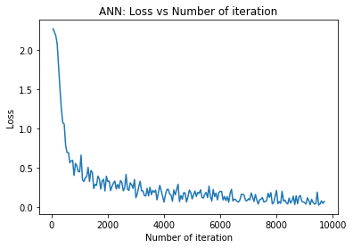
# visualization loss
plt.plot(iteration_list,loss_list)
plt.xlabel("Number of iteration")
plt.ylabel("Loss")
plt.title("ANN: Loss vs Number of iteration")
plt.show()
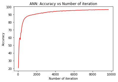
# visualization accuracy
plt.plot(iteration_list,accuracy_list,color = "red")
plt.xlabel("Number of iteration")
plt.ylabel("Accuracy")
plt.title("ANN: Accuracy vs Number of iteration")
plt.show()
Convolutional Neural Network (CNN)
CNN hoạt động rất tốt trong bài toán phân loại ảnh.
Nếu chưa biết về CNN các bạn có thể xem tại đây.
Các bước implement CNN:
- Import thư viện
- Xử lý Dataset
- Hoàn toàn giống với các phần trước.
- Chỉ cần train_loader và test_loader.
- Convolutional layer:
- Tạo feature với filters(kernels).
- Padding: Sau khi qua các filters, các chiều của ảnh ban đầu bị giảm xuống. Tuy nhiên, ta muốn giữ được càng nhiều thông tin càng tốt từ image gốc. TA có thể áp dụng kĩ thuật padding để tăng chiều của feature map sau khi qua convolution layer.
- Ta sử dụng 2 convolutional layer.
- Số feature map là out_channels = 16
- Filter(kernel) size là 5 * 5
- Pooling layer:
- 2 pooling layer mà ta sẽ sử dụng max pooling.
- Pooling size là 2 * 2
- Flattening: Như một cách làm phẳng feature map để làm đầu vào của FC layer.
- Fully Connected Layer:
- Phần này chính là mạng ANN mà ta đã học ở phần trước.
- Ta sẽ không sử dụng activation function tại fully connected layer.
- Bạn có thể nghĩ rằng fully connected layer là logistic regression.
- Ta kết hợp convolutional và logistic regression để tạo ra CNN model.
- Khởi tạo Model Class
- Tạo model
- Loss Class
- Sử dụng Cross entropy loss
- Và nó cũng chứa softmax(logistic function).
- Optimizer Class
- SGD Optimizer
- Traning Model
- Prediction
# Import Libraries
import torch
import torch.nn as nn
import torchvision.transforms as transforms
from torch.autograd import Variable
# Create CNN Model
class CNNModel(nn.Module):
    def __init__(self):
        super(CNNModel, self).__init__()

        # Convolution 1
        self.cnn1 = nn.Conv2d(in_channels=1, out_channels=16, kernel_size=5, stride=1, padding=0)
        self.relu1 = nn.ReLU()

        # Max pool 1
        self.maxpool1 = nn.MaxPool2d(kernel_size=2)

        # Convolution 2
        self.cnn2 = nn.Conv2d(in_channels=16, out_channels=32, kernel_size=5, stride=1, padding=0)
        self.relu2 = nn.ReLU()

        # Max pool 2
        self.maxpool2 = nn.MaxPool2d(kernel_size=2)

        # Fully connected 1
        self.fc1 = nn.Linear(32 * 4 * 4, 10)

    def forward(self, x):
        # Convolution 1
        out = self.cnn1(x)
        out = self.relu1(out)

        # Max pool 1
        out = self.maxpool1(out)

        # Convolution 2
        out = self.cnn2(out)
        out = self.relu2(out)

        # Max pool 2
        out = self.maxpool2(out)
        out = out.view(out.size(0), -1)

        # Linear function (readout)
        out = self.fc1(out)

        return out

# batch_size, epoch and iteration
batch_size = 100
n_iters = 2500
num_epochs = n_iters / (len(features_train) / batch_size)
num_epochs = int(num_epochs)

# Pytorch train and test sets
train = torch.utils.data.TensorDataset(featuresTrain,targetsTrain)
test = torch.utils.data.TensorDataset(featuresTest,targetsTest)

# data loader
train_loader = torch.utils.data.DataLoader(train, batch_size = batch_size, shuffle = False)
test_loader = torch.utils.data.DataLoader(test, batch_size = batch_size, shuffle = False)

# Create ANN
model = CNNModel()

# Cross Entropy Loss
error = nn.CrossEntropyLoss()

# SGD Optimizer
learning_rate = 0.1
optimizer = torch.optim.SGD(model.parameters(), lr=learning_rate)
# CNN model training
count = 0
loss_list = []
iteration_list = []
accuracy_list = []
for epoch in range(num_epochs):
    for i, (images, labels) in enumerate(train_loader):

        train = Variable(images.view(100,1,28,28))
        labels = Variable(labels)

        # Clear gradients
        optimizer.zero_grad()

        # Forward propagation
        outputs = model(train)

        # Calculate softmax and ross entropy loss
        loss = error(outputs, labels)

        # Calculating gradients
        loss.backward()

        # Update parameters
        optimizer.step()
        count += 1
        if count % 50 == 0:
            # Calculate Accuracy
            correct = 0
            total = 0
            # Iterate through test dataset
            for images, labels in test_loader:

                test = Variable(images.view(100,1,28,28))

                # Forward propagation
                outputs = model(test)

                # Get predictions from the maximum value
                predicted = torch.max(outputs.data, 1)[1]

                # Total number of labels
                total += len(labels)

                correct += (predicted == labels).sum()

            accuracy = 100 * correct / float(total)

            # store loss and iteration
            loss_list.append(loss.data)
            iteration_list.append(count)
            accuracy_list.append(accuracy)
            if count % 500 == 0:
                # Print Loss
                print('Iteration: {}  Loss: {}  Accuracy: {} %'.format(count, loss.data[0], accuracy))
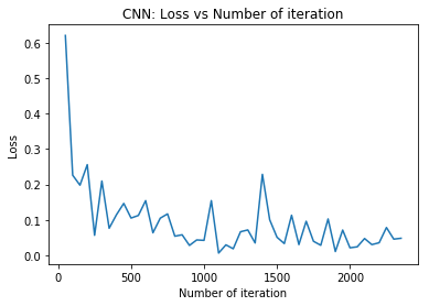
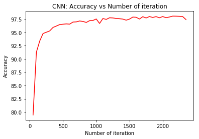
Iteration: 500  Loss: 0.10512177646160126  Accuracy: 96.53571428571429 %
Iteration: 1000  Loss: 0.042111221700906754  Accuracy: 97.52380952380952 %
Iteration: 1500  Loss: 0.05093002691864967  Accuracy: 97.5 %
Iteration: 2000  Loss: 0.021129857748746872  Accuracy: 97.97619047619048 %
# visualization loss
plt.plot(iteration_list,loss_list)
plt.xlabel("Number of iteration")
plt.ylabel("Loss")
plt.title("CNN: Loss vs Number of iteration")
plt.show()

# visualization accuracy
plt.plot(iteration_list,accuracy_list,color = "red")
plt.xlabel("Number of iteration")
plt.ylabel("Accuracy")
plt.title("CNN: Accuracy vs Number of iteration")
plt.show()
Hy vọng rằng sau 2 phần về làm quen với pytorch các bạn đã có thể code quen tay hơn và sử dụng thành thục pytorch trong việc tạo ra các model đơn giản. Trên đây là những model hết sức đơn giản trong Machine learning nhưng mình tin là khi thành thục nó bằng pytorch thì việc các bạn học cách implement nhiều mạng khác sẽ dễ dàng hơn rất nhiều.
- https://www.kaggle.com/kanncaa1/pytorch-tutorial-for-deep-learning-lovers